Code
library(katex)
library(gt)
library(gtsummary)
library(devtools)
library(MEPS)
library(tidyverse)library(katex)
library(gt)
library(gtsummary)
library(devtools)
library(MEPS)
library(tidyverse)In this presentation, we will be discussing how to use the Generalized Linear Model (GLM) method using count data in the R programming language. We will show how to clean and wrangle the data, show necessary columns to execute our method, discuss assumptions held, showcase the code used to run this GLM, and the interpretation of our output results.
As you know, a simple linear regression has two major components: a Y, dependent outcome and an X, which is your independent or your predictor variable. the model looks something like this:
E(Y|X) = \beta_0 + \beta_1 where \beta_0 is your intercept and \beta_1 is your slope. A linear model is a function, that us used to fit a data. We often use this method to see the association, or strength in association between two variables of interest:
# load data:
data(trees)

#rename variables:
names(trees) <- c("DBH_in","height_ft", "volume_ft3")

# simple model:
model <- lm(DBH_in ~ height_ft, data = trees)

# plot:
simple_trees <-
  #data
  ggplot(data = trees) +

  # x and y
  aes(x = height_ft, y = DBH_in) +

  #labels
  labs(title = "Example of Simple Association - Using Trees Data",
       x = "Height in feet",
       y = "Diameter in inches") +

  # add points
  geom_point() +

  # add the lm
  geom_smooth(method = "lm", color = "blue", se = FALSE) +

  # add a simple theme
  theme_bw()

# actual plot:
simple_trees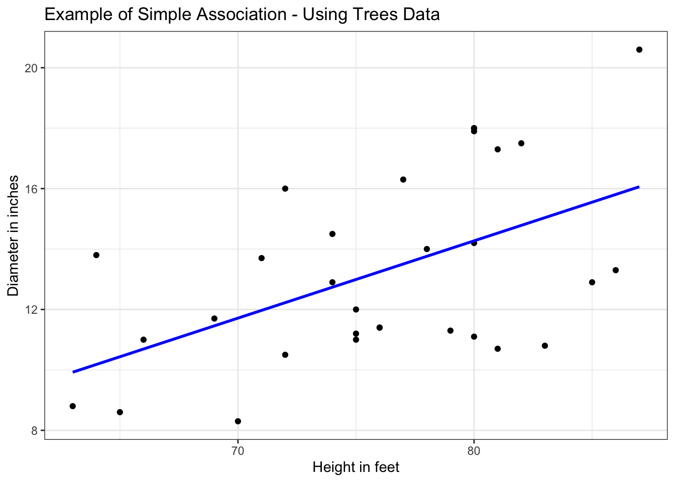
Often you will find this model writen in this form:
E(Y|X) = \beta_0 + \beta_1 + \varepsilon where \beta_0 and \beta_1 are our coefficients that need to be estimated and \varepsilon, or the error term, is used for more complex lines. Our goal is to see the association between an outcome with an exposure.
Before diving into the generalized models, lets quickly overview the assumptions of linear regression.
Something to note, that in the simple explanation above we are assuming our Y variable (remember one of the points we talked above above? that y holds a specific distribution!) is continuous. So lets talk about our Y variable having a count distribution.
the term “generalized” is a big umbrella term used to describe a large class of models. Our response variable y_i is following an exponential family distribution with a mean of u_i which is sometimes non-linear! However McCallagh and Nelder considered them to be linear because our covariate affect the distribution of y_i only through linear combination.
there are three major components of a GLM:
log(\pmb{\mu}) = \alpha + \beta_1x_1 + ... B_nx_n + \epsilon
a Poisson regression models how the mean of a discrete (or we can say count too!) response variable Y depends on our explanatory X variables. Here is a simple look at the Poisson regression:
log \lambda_i = \beta_0 + \beta x_i where the random component: the distribution of Y is the mean of \lambda and the systematic component is the explanatory variable (or your X variables, which can be continuous or categorical) that is linearly associated. Or can be transformed if non-linear, and the link function is the log link stated in the section above (link the section number here?)
An advantage of using GLM over a normal line model is the link function gives us more flexibility in modeling and this model uses the Maximum likelihood estimate. Additionally we can use different inference tools like Wald’s test for logistic and Poisson models.
\pmb{\mu} = exp(\alpha + \beta x) = e^\alpha (e^\beta)^x where one unit increase in X has a multiplicative impact on your e^\beta power on the mean. (More on this a little later in the interpretation section!)
Like with different models in statistics, one must follow the assumptions of a regression, and yes, Poisson has them as well. The assumptions for a Poisson regression are as follows:
\pmb{\mu} = E(X) = \lambda \sigma^2 = \lambda
when your modeling count data, the link scale is linear. So the effects are additive on the link. While your response scale is nonlinear (this is on the exponent) and so the effects are multiplicative. makes sense? we will work out an example now!
Lets import the built in National Health Care Survery data set from the Medical Expenditure Panel Survey website located here. the code book can also be located here for the 2020 Full year Consolidate data file.
# clean
HC2020_clean <- read_csv("/Users/anbravo/GitHub/R-health-blog/HC2020_clean.csv")

# Load data from AHRQ MEPS website
hc2020 = read_MEPS(file = "h224")

# lets name a copy of this data set so i don't ruin it
hc2020_2 <- hc2020

# these variables are upper case, lets turn them lower case
names(hc2020_2) <- tolower(names(hc2020_2))

# theres about 14,000 variables. lets keep the ones we want to look at
hc2020_subset <- hc2020_2 |>
  select(dupersid,obdrv20, ertot20, rthlth31, adpain42, region31, age20x, racev1x, sex, marry31x, educyr, faminc20, empst31, mcare20)


# cleaning names:--------------------------------------------------------------
# dupersid = Person ID
# obdrv20 = number of office based physician visits in 2020
# ertot20 = emergency rooms visits in 2020
# rthlth31 = perceived health status
# adpain41 = pain level
# region31 = Census region: Northest, midwest, south and west
# age20x = Age as of Dec 2020
# racev1x = race: white, black, American indiain, Asian, multiple races
# sex = sex at birth
# marry31x = marital status
# educyr = year of ed when entered in MEPS
# faminc20 = family total income
# empst31 = employment status
# mcare20 = Covered by medicare? Yes/no

# removing old names because that sub header in columns messes me up sometimes ---

names(hc2020_subset) <- NULL


new_names <- c("Person_ID",
               "Nubr_office_visits",
               "Nubr_emergency_visits",
               "Health_status",
               "Pain_Level",
               "Region",
               "Age_as_Dec2020",
               "Race",
               "Is_male",
               "Is_married",
               "Education_lvl",
               "Total_fam_incom",
               "Is_employed",
               "Covered_by_MediCar")


names(hc2020_subset) <- new_names


# this data set has codes for NA, will switch to NA in R ------------------------

HC2020_clean <- HC2020_clean |>
  mutate(Pain_Level = na_if(Pain_Level, -15)) |>
  mutate(Health_status = na_if(Health_status, -8)) |>
  mutate(Region = na_if(Region, -1)) |>
  mutate(Age_as_Dec2020 = na_if(Age_as_Dec2020, -1)) |>
  mutate(Is_married = na_if(Is_married,-8 )) |>
  mutate(Is_employed = na_if(Is_employed, -15)) |>
  mutate(Education_lvl = na_if(Education_lvl, -15)) |>
  mutate(Covered_by_MediCar = na_if(Covered_by_MediCar, -1))


# also, for ease of interpretation i will dichotomize some variables ------------


 HC2020_clean <- HC2020_clean |>
  mutate(Is_married = ifelse(Is_married == 1, 1, 0)) |>
  mutate(Is_employed = ifelse(Is_employed == 1, 1, 0)) |>
  mutate(Is_male = ifelse(Is_male == 1 , 1, 0 )) |>
  mutate(Covered_by_MediCar = ifelse(Covered_by_MediCar == 1, 1, 0))


# i also want to transform some variable using case when -----------------------

HC2020_clean <- HC2020_clean |>
  mutate(Health_status = case_when(
    Health_status == 1 ~ "Good",
    Health_status == 2 ~ "Good",
    Health_status == 3 ~ "Fair",
    Health_status == 4 ~ "Fair",
    Health_status == 5 ~ "Poor"
    ))

# i want to write CSV this data set for later use --------------------------------

write_csv(hc2020_subset,
          file = "/Users/anbravo/GitHub/R-health-blog/HC2020_clean.csv")
let’s say i want to take a sneak peak at this data set. I will use the gtsummary package to look at the first levels of the data set, and I just want to very simply make this data set interactive by using the opt_interactive() function in the gt package.
HC2020_clean |>
  select(Person_ID, Nubr_office_visits, Health_status, Pain_Level, Region, Is_employed, Is_married, Is_employed) |>
  #head(10) |>
  gt() |>

  tab_header(
    title = "Brief view of HC 2020 data set",
    subtitle = "2020 Data from MEPS website"
  ) |>

 opt_interactive(
   use_search = TRUE,
   use_highlight = TRUE,
   use_compact_mode = TRUE,
   use_resizers = TRUE,
   use_text_wrapping = FALSE,
   pagination_type = "jump"
)Remember what I said earlier about the mean and variance being the same? EDA is important because it might tell us more details about our variable of interest. For this particular question, we might be interested in the number of times an event has occurred. In this case, the number of times someone pay a visit to an office doctor. This data follows everyone for exactly one year.
Because we are looking at count data, we might find it important to check out the mean and variance of our Y variables. In the case that our Y variable mean and variance are not the same, we might consider some sort of transformation. Transforming a data set can help with the normality of it.
mean(HC2020_clean$Nubr_office_visits, na.rm = TRUE)[1] 2.792591the mean of this data set is about 2.79.
var(HC2020_clean$Nubr_office_visits, na.rm = TRUE)[1] 34.58851and the variance is about 34.59. We might need to do something with this particular data set but as an example, lets first run a Generalized Linear Model without doing any kind of transformation to the data.
The basic core functions of a GLM look something like this: glm(counts ~ outcome + treatment, data = data_set, family = poisson() which includes:
counts: would be your Y variabledata: where your pulling the data from~: or an equal signoutcome + treatment: are your X variablesfamily: the link or distribution you are followingWe are interested in measuring number of visits to a doctors office as a function of perceived health, sex assigned at birth, and marital status.
# build first model
PossionModel1 <- glm(Nubr_office_visits ~ Health_status + Is_male + Is_married,
                     data = HC2020_clean, family = "poisson")

# check summary
summary(PossionModel1)
Call:
glm(formula = Nubr_office_visits ~ Health_status + Is_male +
    Is_married, family = "poisson", data = HC2020_clean)

Deviance Residuals:
   Min      1Q  Median      3Q     Max
-4.575  -2.069  -1.227   0.310  34.409

Coefficients:
                   Estimate Std. Error z value Pr(>|z|)
(Intercept)        1.340582   0.006745  198.76   <2e-16 ***
Health_statusGood -0.579132   0.007486  -77.37   <2e-16 ***
Health_statusPoor  0.749656   0.014752   50.82   <2e-16 ***
Is_male           -0.296143   0.007366  -40.20   <2e-16 ***
Is_married         0.258006   0.007280   35.44   <2e-16 ***
---
Signif. codes:  0 '***' 0.001 '**' 0.01 '*' 0.05 '.' 0.1 ' ' 1

(Dispersion parameter for poisson family taken to be 1)

    Null deviance: 164561  on 27182  degrees of freedom
Residual deviance: 151166  on 27178  degrees of freedom
  (622 observations deleted due to missingness)
AIC: 199315

Number of Fisher Scoring iterations: 6
this summary gives us the null deviance, which is the total sum of squares, and the residual deviance which is the sum of square errors or the unexplained deviance. We also get the AIC for this model (although AIC is more useful when comparing to other model fits) and we also get the model coefficients for Health status, sex assigned at birth, and marital status.
Additionally, this output is extremely ugly so we will feed this model into gtsummary in a little bit so looks a little better.